CRM
Salesforce Backs Out of Informatica Deal, Reports
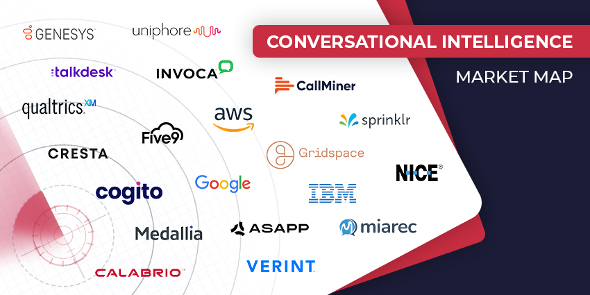
Speech Analytics
The Top Conversational Intelligence Vendors for 2024
Text Analytics
SMS Vulnerabilities: Weaknesses That Consumers & Enterprises Must Be Aware Of
Contact Centre
Omnichannel Contact Center: The Hot Trends of 2024
CRM Excellence Unleashed: The Ultimate Guide on How to Use CRM Effectively
Mastery in Motion: Defining Process Knowledge with Examples and Best Practices
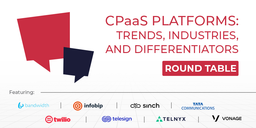
CPaaS Platforms: Trends, Industries, and Differentiators
Loyalty Management
How to Handle Difficult Customers? 10 Strategies for Navigating the Storm
CX TV
Customer Contact Week 2024: What to Expect from the World’s Largest Customer Contact Event
The Google-HubSpot Acquisition Rumors: Could It Really Happen?
Klarna’s Bot Does the Work of 700 Full-Time Contact Center Agents. Could Yours?
BIG CX News – Enterprise Connect 2024: The Roundup ft. Five9, Cisco, Salesforce & More
Content Guru Confirms $150MN CCaaS Megadeal, the Biggest of 2023